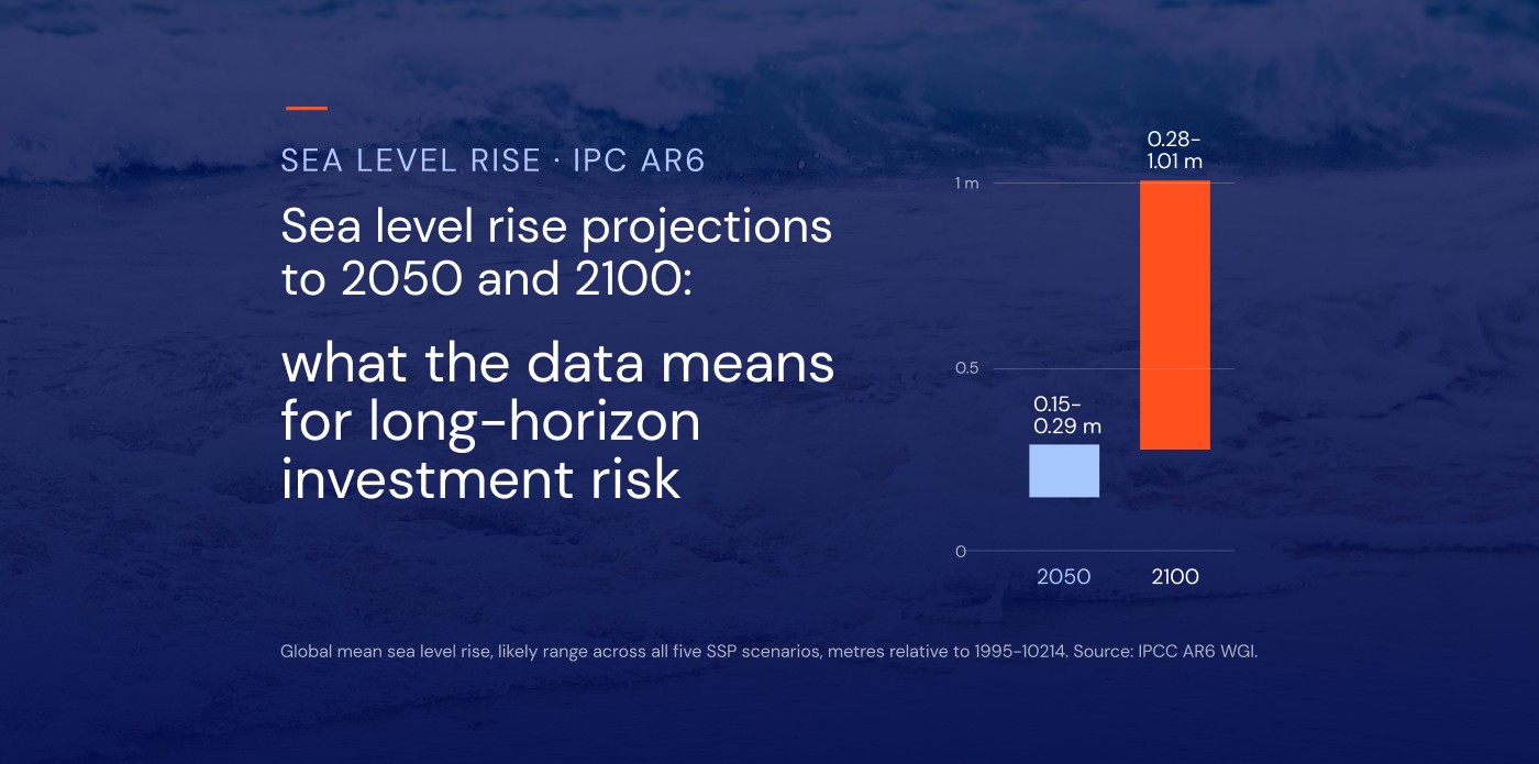
How much will the sea rise by 2050? The IPCC's Sixth Assessment Report (AR6) gives the estimated sea level rise by 2050 as roughly 15 to 29 cm of global mean sea level rise, measured against the 1995–2014 average. That range holds across every emissions scenario the IPCC assessed.

For anyone allocating capital over long horizons, that figure is only the starting point. The financial estimates are far less settled, and far larger. Across the world’s 136 largest coastal cities, average annual flood losses estimated at about US$6 billion in 2005 are projected to reach US$60–63 billion a year by 2050, even if flood defences are upgraded to keep flood probabilities constant. The more useful information sits in two places: how the projections spread apart after 2050, and how far the figure for a specific coastline sits from the global average.

This article sets out what AR6 projects to 2050 and 2100, why projections are not predictions, and how each part of the curve maps onto hold periods, loan tenors and asset lives. For a visual view of exposure by location, see our sea level rise map article.

Estimated sea level rise by 2050: what the data says

IPCC AR6 projects global mean sea level rise of roughly 0.15 to 0.29 m by 2050, relative to 1995–2014, across all five core emissions scenarios. These are the IPCC’s likely ranges, meaning there is roughly a two-in-three chance the outcome falls within them. 

The most useful detail is how closely the scenarios agree. Under a very low emissions pathway, the likely range for 2050 is 0.15 to 0.23 m. Under a very high one, it is 0.20 to 0.29 m. The ranges overlap almost entirely.

The reason is physical. Most of the projected sea level rise by 2050 is driven by warming already in the climate system: oceans continue to expand as they absorb heat, and glaciers and ice sheets respond slowly to temperatures that have already been reached. Emissions cuts made today change the trajectory, but their effect on sea level shows up mainly in the second half of the century.

Two points matter when using these figures:

• The baseline is 1995–2014, not today. Part of the projected rise to 2050 has already happened. The figures should never be read as additional rise from now.
• They describe a global average. Regional assessments can give higher figures because of local factors. NOAA's 2022 interagency technical report, for example, projects 0.25 to 0.30 m of rise along the contiguous US coastline between 2020 and 2050, using a different baseline and method.

So the 2050 answer is fairly settled. The questions that matter for investors start after it.

IPCC AR6 sea level rise projections to 2100: where scenarios diverge

By 2100, the choice of scenario changes the answer substantially. AR6 uses Shared Socioeconomic Pathways (SSPs), which combine an emissions trajectory with assumptions about population, economic growth and policy. They succeed the Representative Concentration Pathways (RCPs) used in earlier reports.

‍

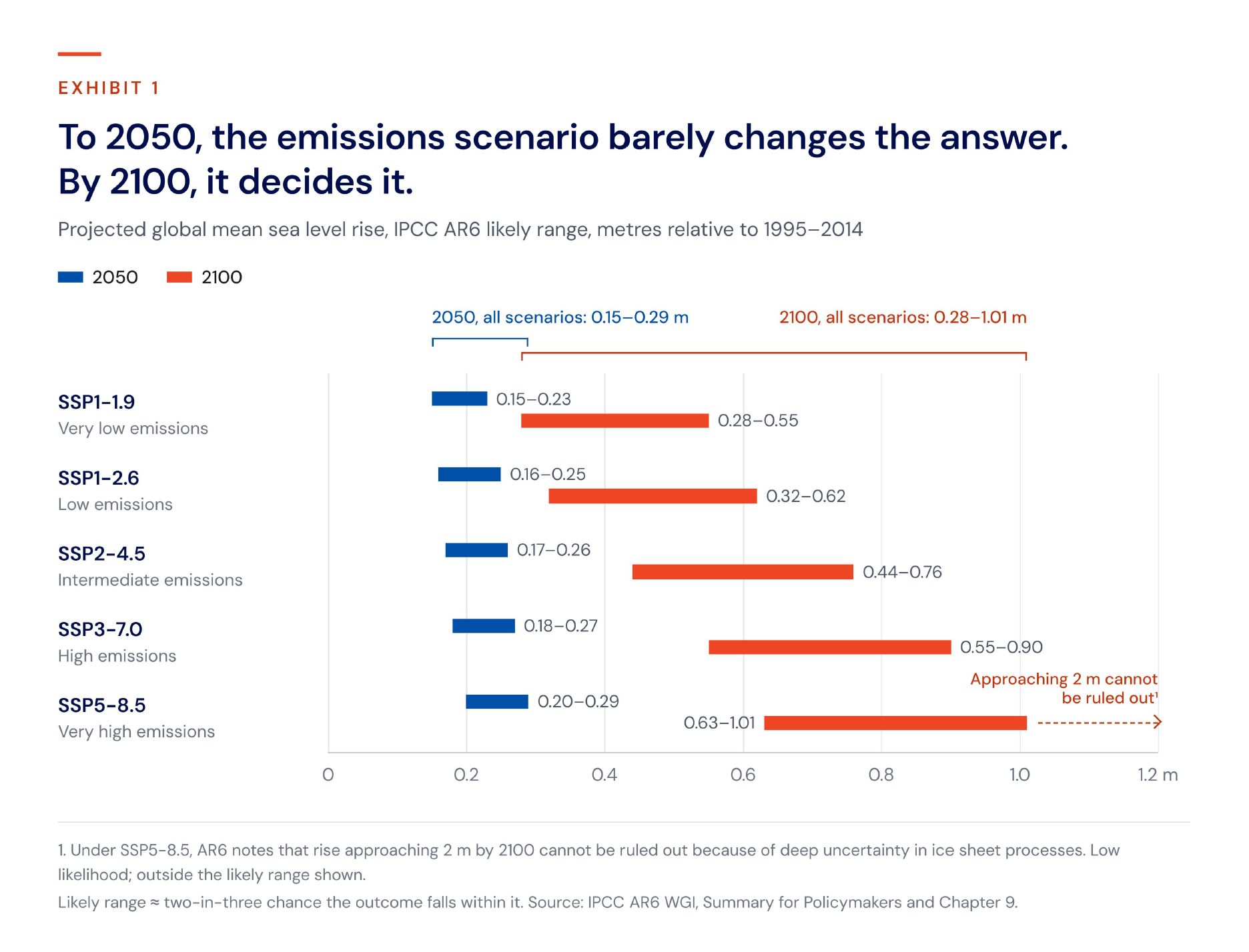
In 2050, the gap between the lowest and highest scenario is a few centimetres. By 2100, the upper end of the very high scenario is almost double that of the very low one.

The likely ranges also leave out processes the IPCC could not assess with confidence, chiefly the potential for rapid ice sheet instability in Antarctica. Under SSP5-8.5, AR6 notes that rise approaching 2 m by 2100 cannot be ruled out because of this deep uncertainty. This is best treated as a stress-test scenario, not a forecast: low likelihood, but high impact for assets designed to last.

Nor does the curve stop in 2100. Sea level will keep rising for centuries to millennia under every scenario, because the deep ocean and ice sheets take a long time to reach equilibrium.

Sea level rise predictions vs. projections: why the distinction matters

Sea level rise predictions are what most searches ask for, but what the IPCC publishes are projections. The difference is practical, not semantic.

A prediction states what will happen. A projection states what would happen if a given set of assumptions holds: a particular path for emissions, land use and the climate system's response. Each AR6 figure is conditional on its scenario. None of them is a forecast of the most probable future.

For investors, this changes how the numbers should be used. Rather than picking one figure and planning around it, treat the scenarios as a range of plausible futures and test assets and portfolios against several of them.

The ranges themselves need care too. A likely range covers roughly two-thirds of the probability, which leaves a real chance that the outcome falls outside it, in either direction. For an asset with a 40-year life, the upper tail often matters more than the median, because that is where losses concentrate.

This is also a useful test for any climate risk figure presented to an investment committee. A credible number should show its working: which scenario it assumes, which time horizon it covers and how much uncertainty surrounds it. If those three things are not visible, the number is hard to defend in front of auditors, lenders or limited partners.

Why the global average is the wrong number for an asset

A port, a substation or a coastal logistics park does not experience global mean sea level. It experiences relative sea level at its own location, and that can differ from the global figure by a wide margin. Three factors explain most of the gap.

Regional ocean and gravitational effects. Sea level does not rise evenly. Ocean currents, wind patterns and differences in water temperature and salinity redistribute water across basins. As ice sheets lose mass, their gravitational pull on nearby ocean weakens, so sea level near a melting ice sheet can rise less than average while distant coastlines rise more.

Vertical land motion. The land itself moves. Subsiding river deltas and coastal cities built on compacting sediment, or where groundwater is extracted, can see relative rise well above the global mean. Parts of northern Europe and Canada are still rising after the last ice age, which offsets some or all of the rise in the sea. For an asset, the relevant figure is the sea relative to the land it stands on. 

Extreme sea levels. Most damage comes from storm surges and high tides, not from the slow change in the average. A modest rise in mean sea level lifts the base on which every extreme event sits, so floods that were once rare become routine. AR6 projects that extreme sea levels that occurred once a century in the recent past will occur at least once a year at more than half of all tide gauge locations by 2100.

This is why return periods matter more than mean rise for most asset decisions. A change from a 1-in-100-year event to a 1-in-5-year event alters design standards, insurance terms and operating costs long before the average shifts noticeably. Our sea level rise map article shows how this varies by coastline.

What sea level rise could cost: the financial estimates

Physical projections tell you how far the sea may rise. Financial estimates show what that means for losses, and they vary far more, because they depend on emissions, on asset values and, above all, on how much flood protection is built.

Coastal cities to 2050. A study of 136 major coastal cities, led by World Bank economist Stéphane Hallegatte, estimates that average annual flood losses could reach US$52 billion by 2050 from socio-economic change alone. Adding sea level rise and subsidence takes this to US$60–63 billion a year, and that assumes defences are upgraded. Without upgrades to present protection, losses could reach US$1 trillion or more per year. The study assumed 0.2–0.4 m of mean sea level rise by 2050, close to the upper end of the AR6 range.

Europe to 2100. The European Commission’s Joint Research Centre projects that, without further investment in coastal adaptation, expected annual damage from coastal flooding of €1.25 billion today could rise by two to three orders of magnitude by the end of the century, to between €93 billion and €961 billion. The study identifies climate change as the main driver of the increase, ahead of urbanisation and rising asset values.

Global asset exposure. Under high emissions and with no flood defences, a 2020 study in Scientific Reports estimates that assets exposed to coastal flooding could be worth up to US$14.2 trillion by 2100, around 20% of global GDP. This is a measure of exposure, not losses, and a deliberate upper bound.

The range in these estimates is the point. The gap between a protected and an unprotected coastline, or between an intermediate and a very high scenario, is often larger than the mean rise itself. Investors are not choosing a number. They are choosing which assumptions their capital can live with.

What the data means for long-horizon investment risk

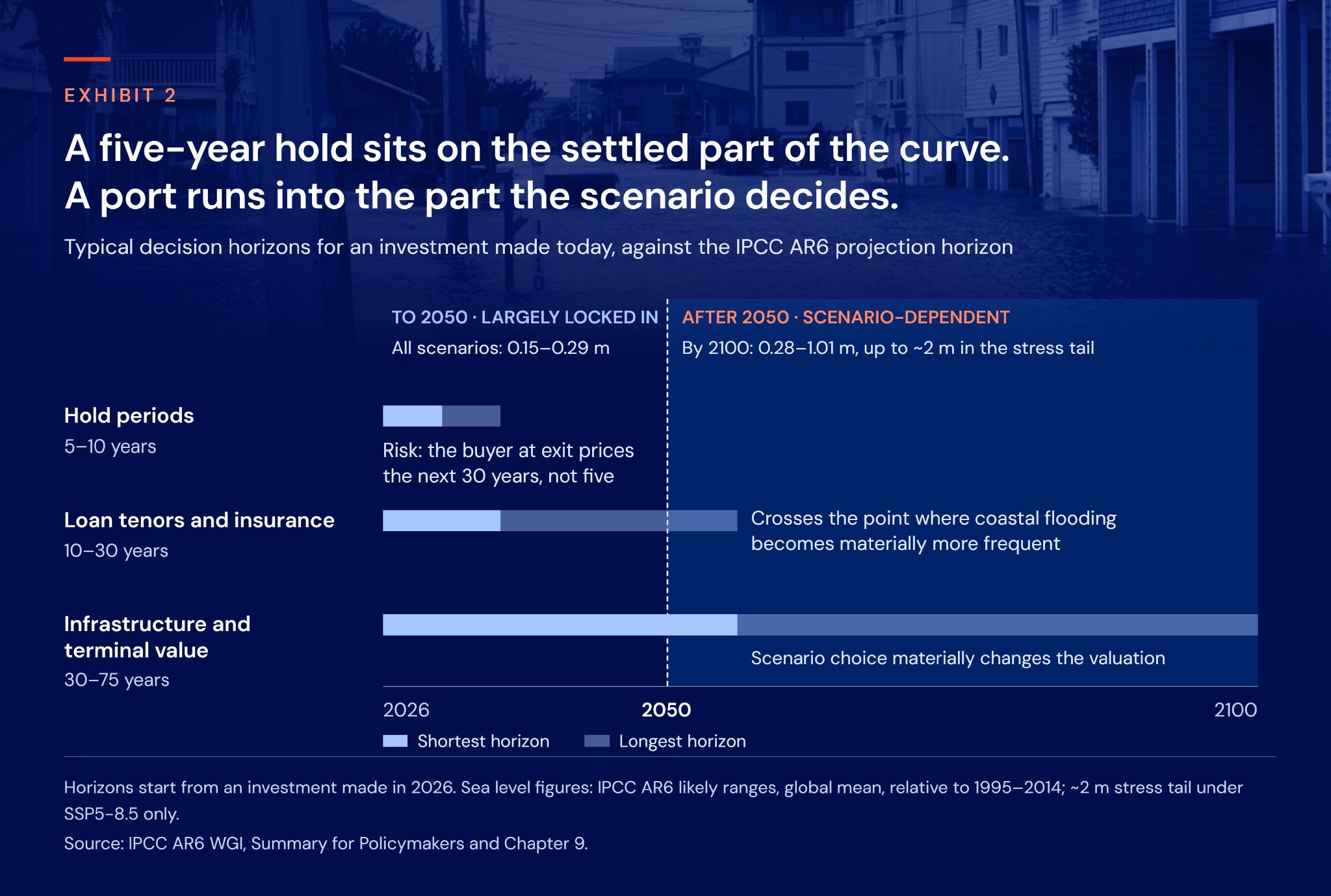
The most practical way to use AR6 projections is to map scenario horizons onto decision horizons. Each type of investment sits on a different part of the curve.

Hold periods (5–10 years)

Over a typical private equity or asset management hold, sea level rise is largely locked in and barely depends on the scenario. The risk here is mispricing what is already coming. The buyer at exit will not be pricing the next five years; they will be pricing the next 30. An asset whose flood exposure becomes visible during the hold can lose value at sale even if nothing has happened to it physically.

Loan tenors and insurance (10–30 years)

A 25-year mortgage or project finance loan written today runs into the period when the frequency of coastal flooding increases materially at many locations. Insurability and premiums can change well within the tenor, which affects collateral values and the borrower's ability to service the debt.

Infrastructure and terminal value (30–75 years)

Ports, energy terminals, water infrastructure and coastal real estate are designed to operate for decades. Their lives extend into the scenario-dependent part of the curve, where the difference between an intermediate and a very high pathway can amount to tens of centimetres of mean rise and a much larger change in extremes. For these assets, scenario choice materially changes the valuation, particularly the terminal value.

‍

Disclosure

IFRS S2 and ESRS E1 both expect companies to assess climate-related risks over short, medium and long-term horizons and to use scenario analysis. Sea level rise is one of the clearest cases where the answer depends on the horizon chosen. Translating that exposure into financial terms, for example through climate value at risk, makes it usable in investment decisions and reporting alike.

What asset-level sea level risk analysis requires

Turning global projections into a figure an investment committee can use takes more than a single number for 2050. A sound analysis should include:

• Local relative sea level, not the global mean, so the figure reflects the coastline and land the asset actually sits on.
• Multiple scenarios, including a stress-test tail, so decisions hold up under more than one plausible future.
• Time steps that match decision horizons, not only 2050 and 2100, so the exposure at exit, at loan maturity and at end of design life can each be assessed.
• Extreme sea levels and return periods, not only mean rise, because extremes drive most of the damage.
• Financial translation and a traceable methodology, so the result can be defended to auditors, lenders and investors.

EarthScan, Mitiga Solutions’ climate risk intelligence platform, is built around these requirements. It combines the CMIP6 global climate models with CORDEX regional models and over 40 years of observational data, and delivers continuous climate data in five-year increments from 1970 to 2100 across multiple scenarios. Results are available at asset level, with return periods for every hazard and climate value at risk to express physical exposure in financial terms. The methodology is backed by more than 300 peer-reviewed publications.

Which part of the curve is your capital on? 

The estimated sea level rise by 2050 is one of the more settled numbers in climate science. That is exactly why, on its own, it says little about investment risk.

What matters is which part of the curve each investment sits on. A five-year hold is exposed to rise that is already locked in, and to how the next owner prices what follows. A 30-year loan crosses the point where coastal floods become far more frequent. A port or energy terminal runs into the decades where the scenario decides the outcome.

‍

See sea level projections at asset level, in five-year steps to 2100

‍

Sources

• IPCC (2021). Climate Change 2021: The Physical Science Basis. Summary for Policymakers. Contribution of Working Group I to the Sixth Assessment Report.
• Fox-Kemper, B. et al. (2021). Chapter 9: Ocean, Cryosphere and Sea Level Change. In: IPCC AR6 WGI.
• Sweet, W.V. et al. (2022). Global and Regional Sea Level Rise Scenarios for the United States. NOAA Technical Report NOS 01.
• NASA. IPCC AR6 Sea Level Projection Tool, for location-specific projections.
• Hallegatte, S. et al. (2013). Future flood losses in major coastal cities. Nature Climate Change, 3, 802–806.
• Vousdoukas, M.I. et al. (2018). Climatic and socioeconomic controls of future coastal flood risk in Europe. Nature Climate Change, 8, 776–780.
• Kirezci, E. et al. (2020). Projections of global-scale extreme sea levels and resulting episodic coastal flooding over the 21st century. Scientific Reports, 10, 11629.
• Bernstein, A., Gustafson, M.T. and Lewis, R. (2019). Disaster on the horizon: the price effect of sea level rise. Journal of Financial Economics, 134(2), 253–272.

‍